Object Estate Table:

Name	Caption
ID_object	ID object
District	District
TypePlan	TypePlan
Rooms	Rooms
FirstLast	FirstLast
Total	Total
Live	Live
Kitchen	Kitchen
Agency	Agency
Condition	Condition
Price	Price

In the Eliminate Outliers node, the set is checked for the presence of outliers and extreme values. The handling method for outliers is set to Leave Unchanged, while for extreme values it's set to Remove Entries.

The settings for the Eliminate Outliers node are as follows:

• the fields Total, Living, Kitchen, Price — are included in the sample.

Models built on neural networks are fairly robust to outliers and extreme values, so no special efforts are required to prepare a sample for them. Nevertheless, it's better to remove extreme values to improve the quality of model training.

The first step towards training a Neural Network (regression) is to define what data is inputted, and what should be outputted. In this example, the output is the forecasted property price, so correspondingly, the input data are those which directly affect the price of the property.

The data was normalized to bring all quantities to a uniform range. If normalization is not performed, input data of different orders will have unequal influence on the neurons, which may lead to incorrect algorithm calculations. It's also necessary to consider that different normalization methods are applied to continuous and discrete types of data.

The normalization settings in the Neural Network (regression) node are as follows:

• fields District, TypePlan, Rooms, FirstLast, Agency, and Condition — Indicator.
• for the rest of the fields, the Normalizer is absent.

The next stage is to split the data into training and testing sets, and choose a method for validating the Neural Network's forecast.

The settings for splitting into sets in the Neural Network (regression) node are as follows:

• For the Training set, the size percentage chosen is 90%.
• For the Test set, the size percentage chosen is 10%.
• Split Method — Random.
• Validation Method — K-fold Cross Validation.
• Sampling Method — Random.
• Folds for Cross-validation — 10.

Whenever any Neural Network settings are changed, retraining is required.

In the remaining setup steps, all parameters are used by default.

The approximation error for each object is calculated using the Calculator node and the RelErr function. The obtained values show how much the calculated values differ from the actual ones, thus giving an idea of the model's quality.

RelErr(price, price_predicted) * 100

The average approximation error of all objects is calculated using the Grouping component.

The setup of the Average Approximation Error node is as follows:

• The Approximation Error (Average) field has been moved to Indicators.

The average approximation error turned out to be around 8%. This is considered a good result (an error of up to 10-12% is acceptable).

The chart is built based on the original (on the abscissa axis) and forecasted cost. The type of plots in both cases is Scatter.

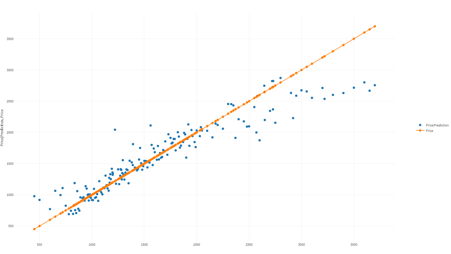
The dispersion of forecasted cost values is concentrated near the original cost values. The diagram vividly demonstrates the quality of Neural Network training and the practical applicability of the model.

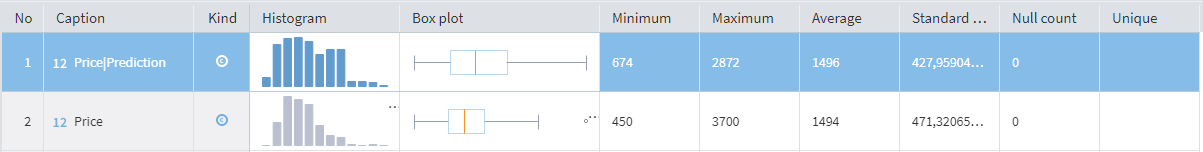
No preliminary settings are required in Statistics. A leftward shift in the histogram indicates that the Neural Network underestimates the forecast for some objects, accordingly, this property will decrease in price.

Detailed forecast values can be viewed in the output data of the Estate value Supernode, using the Table or Quick View visualizers.